Two-step MOR for \(H_\infty\)-robust nonlinear controller design
Jan Heiland (MPI/OVGU Magdeburg)
Amritam Das (TU Eindhoven)
GAMM Annual Meeting at Magdeburg, March 21, 2024
Motivation
The Navier-Stokes equations
\[ \dot v + (v\cdot \nabla) v- \frac{1}{\mathsf{Re}}\Delta v + \nabla p= f, \]
\[ \nabla \cdot v = 0. \]
Control Problem:
- use two small outlets for fluid at the cylinder boundary
- to stabilize the unstable steady state
- with a few point observations in the wake.
Quadratic Stability
The (uncontrolled) Navier-Stokes equations can be realized as an SDC system \[\begin{equation} \dot x(t) = A(x(t))\, x(t), \quad x(0)=x_0 \in \mathbb R^{n}, \end{equation}\] with \(A\colon \mathbb R^{n}\to \mathbb R^{n\times n}\).
Theorem
Quadratic Stability (Prop.
1.1, Shamma 2012):
If there exists \(X>0 \in \mathbb R^{n\times n}\) s. th.
\[\begin{equation}
XA(x) + A(x)^TX < 0
\end{equation}\] along the trajectory \(x\), then the system is asymptotically
stable.
For \(x(t)\in \mathbb R^{n}\), the linear Matrix inequality (LMI) \[\begin{equation} XA(x) + A(x)^TX < 0 \end{equation}\] has to be checked on an infinite set \(\mathcal X\subset \mathbb R^{n}\).
For parametrizations \(x(t) = \Phi\rho(t)\), with \(\rho(t) \in \mathbb R^{r}\), the LMI \[\begin{equation} XA(\Phi \rho) + A(\Phi \rho)^TX < 0 \end{equation}\] has to be checked on an infinite set \(\mathcal R \subset \mathbb R^{r}\).
Polytopic LPV System Approximations
Theorem
Polytopic LPV systems (Apkarian, Gahinet, and Becker 1995):
If \(\tilde A(\rho) :=
A(\Phi\rho)\) is linear, and \(\rho(t)\in R\subset \mathbb R^{r}\) with a
polytope \(R\) of \(N\) vertices \(\rho^{(i)}\), then quadratic
stability holds, if \[\begin{equation}
X\tilde A(\rho^{(i)}) + \tilde A(\rho^{(i)})^TX < 0
\end{equation}\] at the vertices \(\rho^{(i)}\), for \(i=1,\dotsc,N\).
Thus, for polytopic LPV systems, we need to solve an \[\begin{equation} N\cdot n \end{equation}\] dimensional LMI to establish stability.
The direct way (like hinfgs in Matlab) uses the
bounding box for \(\rho\) and
solves a \[
2^{r+1}\cdot n
\] dimensional LMI.
For basic POD (see, e.g., (Hashemi and Werner 2011))
\[\begin{equation} \dot {\hat x} (t) = \hat A(\hat x(t))\, \hat x(t), \quad \hat x(0)=\hat x_0 \in \mathbb R^{k} \end{equation}\]
the LMI to sizes reduces \(2^{k+1}\cdot k\).
However, already for \(k=10\), the LMI size is \(20\ 480\) despite the low accuracy of the model.
Our approach: two level reduction
- Reduce the state-space to a moderate dimension \(k_x\)
- Parametrize the coefficient with very few dimensions \(k_r\).
Then, the system reads \[\begin{equation} \dot {\tilde x} (t) = \tilde A(\rho(\tilde x(t)))\, \tilde x(t), \quad \tilde x(0)=\tilde x_0 \in \mathbb R^{k_x}, \quad \rho(\tilde x(t)) \in \mathbb R^{k_r}, \end{equation}\] and for \(k_x=36\) and \(k_r=6\), the LMI size is \(254\) while accuracy is good.
Illustration of model accuracy via the limit cycles for
- the full order model (top)
- the POD reduction with 10 modes (middle)
- our two-layer approach (bottom row)
How about further reduction?
Critical factor is \(2^{k_r+1}\): the number of vertices of the bounding box for \(\mathcal R \supset \rho\).
Consider a polytope \(\mathcal P\) of less vertices that encloses \(\rho\)
- potentially, we could reduce \(2^{k_r + 1} \leftarrow k_r +1\)
- however, the vertices of such a simplex will be far off the actual values
- so that no feasible solutions for the LMIs may be found
- we use a multiobjective optimization to find a polytope \(\mathcal P\)
- of less vertices
- at less extremal coordinates
3D case illustration
- set of trajectory values
- enclosing bounding box
- enclosing polytope
Note the extremal values in the polytope
Controller Design
Using the hinfgs routine from the Robust Control
Toolbox
- very basic implementation of the LMI solves
- likely to be deprecated
- little support for general polytopes \(\mathcal P\)
- closed-loop simulations only with bounding boxes
Example case of \(k_x=36\) and \(k_r=6\).
- bounding box – LMI size: \(4608 = 2^7\cdot 36\)
- optimized polytope – LMI size: \(720 = 20\cdot 36\)
We compare the hinfgs runtime against achieved
performance \(\gamma\) of the
controller.
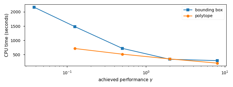
- The polytope representation is generally and significantly faster
- the bounding box achieves a better \(H_\infty\) performance
Conclusion
Promising two-layer reduction for \(H_\infty\) robust gain scheduling for nonlinear systems
Major issue – solving the LMIs
- theoretical complexity
- unsufficient implementations
Future Work
combine model order reduction and controller design in polytopes (see contribution by Yongho Kim)
call on more recent implementations like in LPVcore
do the system theory (PhD student wanted)